This was written with help from AI. Point out errors and earn money! 💰

Understanding the Function $f(x)=\frac{1}{x}$

The function $f(x)=\frac{1}{x}$ is a classical example of a rational function, which is any function that can be written as the ratio of two polynomial functions.

Plotting the Function

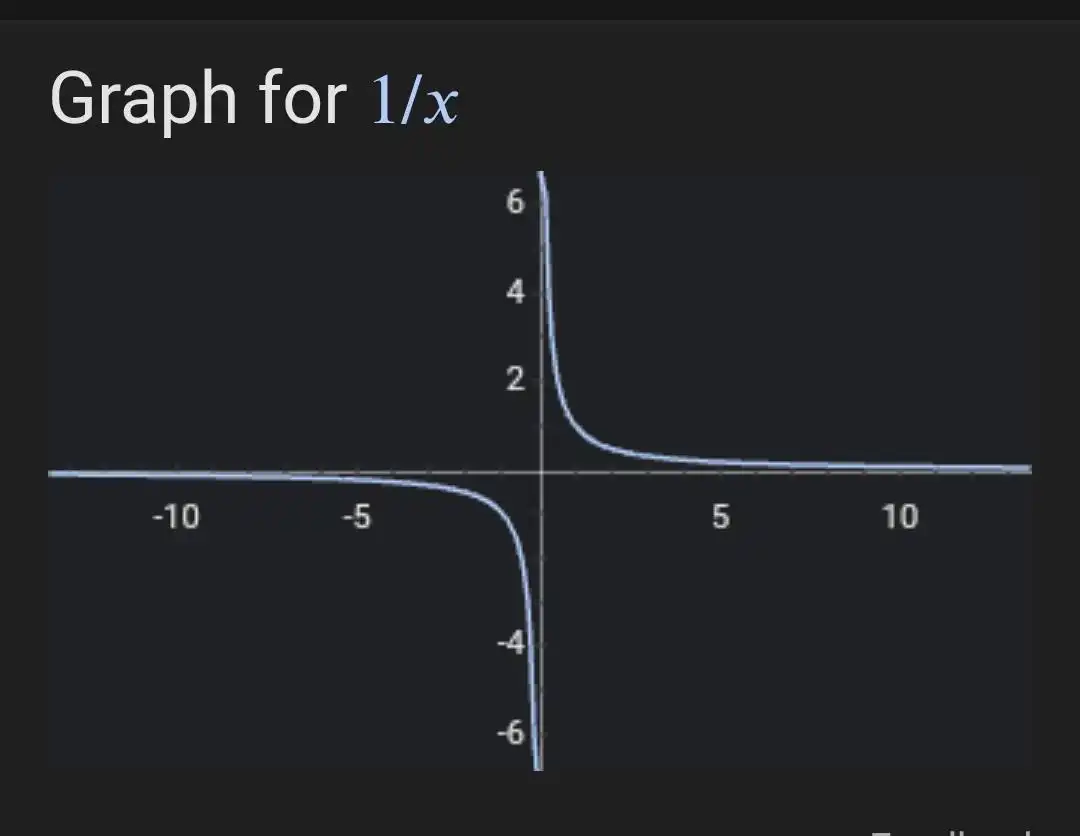
If we plot $f(x)=\frac{1}{x}$, we will notice that the graph divides into two distinct parts, or branches, which are located in different quadrants:

• The first branch is in the first quadrant (top-right) for $x>0$.
• The second branch is in the third quadrant (bottom-left) for $x<0$.

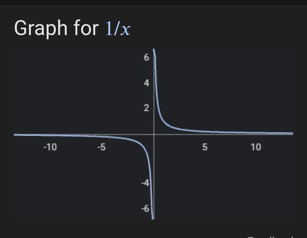
This happens because the denominator $x$ could be either positive or negative.

Asymptotes

Asymptotes are lines that a graph approaches as $x$ tends to infinity or negative infinity.

The above was a poor definition from GPT. Here is a more precise and rigorous definition:

You're correct, the definition I provided was more of an intuitive one. A more precise, mathematical definition is as follows:

An asymptote is a line, such that the distance between the curve and the line approaches zero as they tend to infinity.

There are three types of asymptotes: horizontal, vertical, and oblique.

• A horizontal asymptote, $y=b$, is a horizontal line that the graph of the function $f(x)$ approaches as $x\to +\infty$ or $x\to -\infty$.
• A vertical asymptote, $x=a$, is a vertical line which the graph of the function $f(x)$ approaches as $x\to a^{-}$ (from the left) or $x\to a^{+}$ (from the right).
• An oblique (or slant) asymptote is a line that the graph of the function $f(x)$ approaches as $x\to +\infty$ or $x\to -\infty$, and the line is neither horizontal nor vertical.

In all these cases, the formal definition involves a limit. For example, the line $y=b$ is a horizontal asymptote of $f(x)$ if either

or

For $f(x)=\frac{1}{x}$, there are two asymptotes:

1. Vertical asymptote at $x=0$: The function becomes undefined at $x=0$ since division by zero is undefined in mathematics. As $x$ approaches zero from the left or the right, $f(x)$ tends towards negative or positive infinity respectively. This creates a vertical asymptote at $x=0$.

2. Horizontal asymptote at $y=0$: As $x$ goes to positive or negative infinity, the value of $\frac{1}{x}$ approaches zero, creating a horizontal asymptote at $y=0$.

Calculus of $f(x)=\frac{1}{x}$

Derivative

The derivative of a function measures how the function changes as its input changes. For the function $f(x)=\frac{1}{x}$, its derivative $f^{\prime }(x)$ is given by the following expression:

The negative sign indicates that the function is decreasing as $x$ increases. It's an interesting function - as $x$ goes from $-\infty$ to zero, $y$ goes from zero to $-\infty$ 🤔

Integral

The integral of a function provides the area under the curve of the function. The indefinite integral (antiderivative) of $f(x)=\frac{1}{x}$ is:

where $C$ is the constant of integration.

Properties and Behavior

Finally, let's mention some properties and behavior of this function:

• The function $f(x)=\frac{1}{x}$ is neither an even function nor an odd function. An even function is symmetric about the y-axis, and an odd function is symmetric about the origin. This function is symmetric with respect to the origin, but because it's not defined at $x=0$, it doesn't fully qualify as an odd function.

• This function is hyperbolic, meaning that its graph forms a hyperbola.

• The function is not defined at $x=0$, and this discontinuity is what forms the vertical asymptote.

• The function $f(x)=\frac{1}{x}$ is a simple example of a reciprocal function, which are functions of the form $f(x)=\frac{1}{g(x)}$ where $g(x)$ is any valid function.

This brief lesson covered the basic properties and calculus of the function $f(x)=\frac{1}{x}$. This function provides a good example of rational functions and illustrates concepts like asymptotes, derivatives, and integrals.

Graphing in Python

You can use libraries like matplotlib and numpy to plot this function. Here's a simple Python script:

import matplotlib.pyplot as pltimport numpy as np # Define the functiondef f(x):    return 1/x # Generate x valuesx = np.linspace(-10, -0.1, 400)x = np.append(x, np.linspace(0.1, 10, 400)) # Generate y valuesy = f(x) # Create the plotplt.figure(figsize=(8, 6))plt.plot(x, y, label="y=1/x")plt.title("Plot of y=1/x")plt.xlabel("x")plt.ylabel("y") # Add a horizontal line at y=0 (x-axis)plt.axhline(0, color='black',linewidth=0.5) # Add a vertical line at x=0 (y-axis)plt.axvline(0, color='black',linewidth=0.5) # Add gridplt.grid(color = 'gray', linestyle = '--', linewidth = 0.5) # Create legendplt.legend() # Show the plotplt.show()

Please note that the function isn't defined at $x=0$, so we split the range into two parts, one for $x<0$ and one for $x>0$. This script also adds axes and a grid to the plot for better visualization.

I'll send the first person to send a picture of this graph 0.3 ZEC :D

Also, can someone double check the integral above and give us the intuition of why this is right or wrong?

Applications

The function $f(x)=\frac{1}{x}$ (a reciprocal function) is a mathematical model that appears in various real-world situations. Here are a few examples:

1. Physics - Harmonic Oscillators: In physics, the period of a simple harmonic oscillator (like a pendulum or a spring-mass system) is proportional to the reciprocal of the square root of the mass. If you have the period T on one axis and mass m on the other, it forms a curve similar to the function $f(x)=\frac{1}{x}$.

2. Economics - Law of Demand: In economics, the law of demand states that the quantity demanded for a good rises as the price falls, assuming all other factors remain constant. This can be graphically represented as a downward sloping curve similar to the reciprocal function. The lower the price (increasing along the x-axis), the higher the quantity demanded (y-axis).

3. Chemistry - Pressure and Volume (Boyle's Law): In chemistry, Boyle's Law states that the pressure of a given amount of gas is inversely proportional to its volume at a constant temperature. This means if you graph pressure (P) against volume (V), you get a hyperbola, which is the same shape as the graph of $f(x)=\frac{1}{x}$.

4. Electronics - Ohm's Law: In electronics, resistance is the reciprocal of conductance. According to Ohm's Law, the current flowing through a conductor between two points is directly proportional to the voltage across the two points, and inversely proportional to the resistance. In other words, if you graph conductance (G) against resistance (R), you get a curve that looks like $f(x)=\frac{1}{x}$.

It's important to note that while these situations may be modeled by reciprocal functions, they might not be exact matches for $f(x)=\frac{1}{x}$. The models are approximations, and many factors in real-world situations can cause deviations from these idealized curves.